
特征提取
数字特征提取
数组型特征可以直接作为特征,但是对于一个多维的特征,某一个特征的取值范围特别大,很可能导致其他特征对结果的影响被忽略,这时候我们需要对数字型特征进行预处理,常见的预处理方式有以下几种。
1.标准化:
>>> from sklearn import preprocessing
>>> import numpy as np
>>> X = np.array([[1.,-1.,2],[2.,0.,0.],[0.,1.,-1.]])
>>> X_scaled = preprocessing.scale(X)
>>> X_scaled
array([[ 0.        , -1.22474487,  1.33630621],
       [ 1.22474487,  0.        , -0.26726124],
       [-1.22474487,  1.22474487, -1.06904497]])
2.正则化
>>> X = [[1.,-1.,2.],[2.,0.,0.],[0.,1.,-1.]]
>>> X_normalized = preprocessing.normalize(X, norm='l2')
>>> X_normalized
array([[ 0.40824829, -0.40824829,  0.81649658],
       [ 1.        ,  0.        ,  0.        ],
       [ 0.        ,  0.70710678, -0.70710678]])
3.归一化
>>> X_train = np.array([[1.,-1.,2.],[2.,0., 0.],[0.,-1.,-1.]])
>>> min_max_scaler = preprocessing.MinMaxScaler()
>>> X_train_minmax = min_max_scaler.fit_transform(X_train)
>>> X_train_minmax
array([[ 0.5       ,  0.        ,  1.        ],
       [ 1.        ,  1.        ,  0.33333333],
       [ 0.        ,  0.        ,  0.        ]])
文本型特征提取
文本型特征提取,本质上是做单词切分,不同的单词当作一个新的特征,以hash结构为例:
>>> measurements=[{'city':'Dubai','temperature':33.},
...     {'city':'London','temperature':12.},
...     {'city':'San Fransisco','temperature':18.}
... ]
键值city具有多个取值,“Dubai”、“London”和“San Fransisco”,直接把每个取值作为新的特征即可。键值temperature是数值型,可以直接作为特征使用。
>>> from sklearn.feature_extraction import DictVectorizer
>>> vec = DictVectorizer()
>>> vec.fit_transform(measurements).toarray()
array([[  1.,   0.,   0.,  33.],
       [  0.,   1.,   0.,  12.],
       [  0.,   0.,   1.,  18.]])
>>> vec.get_feature_names()
['city=Dubai', 'city=London', 'city=San Fransisco', 'temperature']
文本特征提取有两个非常重要的模型。
- 词集模型:单词构成的集合,集合中每个元素都只有一个,即词集中的每个单词都只有一个。
- 词袋模型:如果一个单词在文档中出现不止一次,并统计其出现的次数(频数)。
两者本质上的区别,词袋是在词集的基础上增加了频率的维度:词集只关注有和没有,词袋还要关注有几个。
导入相关的函数库:
>>> from sklearn.feature_extraction.text import CountVectorizer
实例化分词对象:
>>> vectorizer = CountVectorizer(min_df=1)
>>> vectorizer
CountVectorizer(analyzer=u'word', binary=False, decode_error=u'strict',
        dtype=<type 'numpy.int64'>, encoding=u'utf-8', input=u'content',
        lowercase=True, max_df=1.0, max_features=None, min_df=1,
        ngram_range=(1, 1), preprocessor=None, stop_words=None,
        strip_accents=None, token_pattern=u'(?u)\\b\\w\\w+\\b',
        tokenizer=None, vocabulary=None)
将文本进行词袋处理:
>>> corpus = [
...     'This is the first document.',
...     'This is the second second document.',
...     'And the third one.',
...     'Is this the first document?']
>>> X = vectorizer.fit_transform(corpus)
>>> X
<4x9 sparse matrix of type '<type 'numpy.int64'>'
	with 19 stored elements in Compressed Sparse Row format>
获取对应的特征名称:
>>> vectorizer.get_feature_names() == (
...     ['and', 'document', 'first', 'is', 'one',
...      'second', 'the', 'third', 'this'])
True
获取词袋数据,至此我们已经完成了词袋化。但是对于程序中的其他文本,如何使用现有的词袋的特征进行向量化呢?
>>> X.toarray()
array([[0, 1, 1, 1, 0, 0, 1, 0, 1],
       [0, 1, 0, 1, 0, 2, 1, 0, 1],
       [1, 0, 0, 0, 1, 0, 1, 1, 0],
       [0, 1, 1, 1, 0, 0, 1, 0, 1]])
我们定义词袋的特征空间叫做词汇表vocabulary:
>>> vocabulary=vectorizer.vocabulary_
>>> vocabulary
{u'and': 0, u'third': 7, u'this': 8, u'is': 3, u'one': 4, u'second': 5, u'the': 6, u'document': 1, u'first': 2}
针对其他文本进行词袋处理时,可以直接使用现有的词汇表:
>>> new_vectorizer
CountVectorizer(analyzer=u'word', binary=False, decode_error=u'strict',
        dtype=<type 'numpy.int64'>, encoding=u'utf-8', input=u'content',
        lowercase=True, max_df=1.0, max_features=None, min_df=1,
        ngram_range=(1, 1), preprocessor=None, stop_words=None,
        strip_accents=None, token_pattern=u'(?u)\\b\\w\\w+\\b',
        tokenizer=None,
        vocabulary={u'and': 0, u'third': 7, u'this': 8, u'is': 3, u'one': 4, u'second': 5, u'the': 6, u'document': 1, u'first': 2})
TensorFlow中有类似实现:
from sklearn.feature_extraction.text import CountVectorizer
from tensorflow.contrib import learn
MAX_DOCUMENT_LENGTH=100
vocab_processor=learn.preprocessing.VocabularyProcessor(MAX_DOCUMENT_LENGTH)
X_train = np.array(list(vocab_processor.fit_transform(X_train)))
X_test = np.array(list(vocab_processor.transform(X_test)))
数据读取
平时处理数据是,CSV是最常见的格式,文件的每行记录一个向量,其中最后一列为标记。TensorFlow提供了非常便携的方式从CSV文件中读取数据集。
加载对应的函数库:
>>> import tensorflow as tf
>>> import numpy as np
从CSV文件中读取数据:
>>> training_set = tf.contrib.learn.datasets.base.load_csv_with_header(
... filename="iris_training.csv",
... target_dtype=np.int,
... features_dtype=np.float32)
>>> feature_columns = [tf.contrib.layers.real_valued_column("", dimension=4)]
>>> x=training_set.data
>>> y=training_set.target
>>> x
array([[ 6.4000001 ,  2.79999995,  5.5999999 ,  2.20000005],
       [ 5.        ,  2.29999995,  3.29999995,  1.        ],
       [ 4.9000001 ,  2.5       ,  4.5       ,  1.70000005],
       [ 4.9000001 ,  3.0999999 ,  1.5       ,  0.1       ],
       [ 5.69999981,  3.79999995,  1.70000005,  0.30000001],
       [ 4.4000001 ,  3.20000005,  1.29999995,  0.2       ],
       [ 5.4000001 ,  3.4000001 ,  1.5       ,  0.40000001],
       [ 6.9000001 ,  3.0999999 ,  5.0999999 ,  2.29999995],
       [ 6.69999981,  3.0999999 ,  4.4000001 ,  1.39999998],
       [ 5.0999999 ,  3.70000005,  1.5       ,  0.40000001],
       [ 5.19999981,  2.70000005,  3.9000001 ,  1.39999998],
       [ 6.9000001 ,  3.0999999 ,  4.9000001 ,  1.5       ],
       [ 5.80000019,  4.        ,  1.20000005,  0.2       ],
       [ 5.4000001 ,  3.9000001 ,  1.70000005,  0.40000001],
       [ 7.69999981,  3.79999995,  6.69999981,  2.20000005],
       [ 6.30000019,  3.29999995,  4.69999981,  1.60000002],
       [ 6.80000019,  3.20000005,  5.9000001 ,  2.29999995],
       [ 7.5999999 ,  3.        ,  6.5999999 ,  2.0999999 ],
       [ 6.4000001 ,  3.20000005,  5.30000019,  2.29999995],
       [ 5.69999981,  4.4000001 ,  1.5       ,  0.40000001],
       [ 6.69999981,  3.29999995,  5.69999981,  2.0999999 ],
       [ 6.4000001 ,  2.79999995,  5.5999999 ,  2.0999999 ],
       [ 5.4000001 ,  3.9000001 ,  1.29999995,  0.40000001],
       [ 6.0999999 ,  2.5999999 ,  5.5999999 ,  1.39999998],
       [ 7.19999981,  3.        ,  5.80000019,  1.60000002],
       [ 5.19999981,  3.5       ,  1.5       ,  0.2       ],
       [ 5.80000019,  2.5999999 ,  4.        ,  1.20000005],
       [ 5.9000001 ,  3.        ,  5.0999999 ,  1.79999995],
       [ 5.4000001 ,  3.        ,  4.5       ,  1.5       ],
       [ 6.69999981,  3.        ,  5.        ,  1.70000005],
       [ 6.30000019,  2.29999995,  4.4000001 ,  1.29999995],
       [ 5.0999999 ,  2.5       ,  3.        ,  1.10000002],
       [ 6.4000001 ,  3.20000005,  4.5       ,  1.5       ],
       [ 6.80000019,  3.        ,  5.5       ,  2.0999999 ],
       [ 6.19999981,  2.79999995,  4.80000019,  1.79999995],
       [ 6.9000001 ,  3.20000005,  5.69999981,  2.29999995],
       [ 6.5       ,  3.20000005,  5.0999999 ,  2.        ],
       [ 5.80000019,  2.79999995,  5.0999999 ,  2.4000001 ],
       [ 5.0999999 ,  3.79999995,  1.5       ,  0.30000001],
       [ 4.80000019,  3.        ,  1.39999998,  0.30000001],
       [ 7.9000001 ,  3.79999995,  6.4000001 ,  2.        ],
       [ 5.80000019,  2.70000005,  5.0999999 ,  1.89999998],
       [ 6.69999981,  3.        ,  5.19999981,  2.29999995],
       [ 5.0999999 ,  3.79999995,  1.89999998,  0.40000001],
       [ 4.69999981,  3.20000005,  1.60000002,  0.2       ],
       [ 6.        ,  2.20000005,  5.        ,  1.5       ],
       [ 4.80000019,  3.4000001 ,  1.60000002,  0.2       ],
       [ 7.69999981,  2.5999999 ,  6.9000001 ,  2.29999995],
       [ 4.5999999 ,  3.5999999 ,  1.        ,  0.2       ],
       [ 7.19999981,  3.20000005,  6.        ,  1.79999995],
       [ 5.        ,  3.29999995,  1.39999998,  0.2       ],
       [ 6.5999999 ,  3.        ,  4.4000001 ,  1.39999998],
       [ 6.0999999 ,  2.79999995,  4.        ,  1.29999995],
       [ 5.        ,  3.20000005,  1.20000005,  0.2       ],
       [ 7.        ,  3.20000005,  4.69999981,  1.39999998],
       [ 6.        ,  3.        ,  4.80000019,  1.79999995],
       [ 7.4000001 ,  2.79999995,  6.0999999 ,  1.89999998],
       [ 5.80000019,  2.70000005,  5.0999999 ,  1.89999998],
       [ 6.19999981,  3.4000001 ,  5.4000001 ,  2.29999995],
       [ 5.        ,  2.        ,  3.5       ,  1.        ],
       [ 5.5999999 ,  2.5       ,  3.9000001 ,  1.10000002],
       [ 6.69999981,  3.0999999 ,  5.5999999 ,  2.4000001 ],
       [ 6.30000019,  2.5       ,  5.        ,  1.89999998],
       [ 6.4000001 ,  3.0999999 ,  5.5       ,  1.79999995],
       [ 6.19999981,  2.20000005,  4.5       ,  1.5       ],
       [ 7.30000019,  2.9000001 ,  6.30000019,  1.79999995],
       [ 4.4000001 ,  3.        ,  1.29999995,  0.2       ],
       [ 7.19999981,  3.5999999 ,  6.0999999 ,  2.5       ],
       [ 6.5       ,  3.        ,  5.5       ,  1.79999995],
       [ 5.        ,  3.4000001 ,  1.5       ,  0.2       ],
       [ 4.69999981,  3.20000005,  1.29999995,  0.2       ],
       [ 6.5999999 ,  2.9000001 ,  4.5999999 ,  1.29999995],
       [ 5.5       ,  3.5       ,  1.29999995,  0.2       ],
       [ 7.69999981,  3.        ,  6.0999999 ,  2.29999995],
       [ 6.0999999 ,  3.        ,  4.9000001 ,  1.79999995],
       [ 4.9000001 ,  3.0999999 ,  1.5       ,  0.1       ],
       [ 5.5       ,  2.4000001 ,  3.79999995,  1.10000002],
       [ 5.69999981,  2.9000001 ,  4.19999981,  1.29999995],
       [ 6.        ,  2.9000001 ,  4.5       ,  1.5       ],
       [ 6.4000001 ,  2.70000005,  5.30000019,  1.89999998],
       [ 5.4000001 ,  3.70000005,  1.5       ,  0.2       ],
       [ 6.0999999 ,  2.9000001 ,  4.69999981,  1.39999998],
       [ 6.5       ,  2.79999995,  4.5999999 ,  1.5       ],
       [ 5.5999999 ,  2.70000005,  4.19999981,  1.29999995],
       [ 6.30000019,  3.4000001 ,  5.5999999 ,  2.4000001 ],
       [ 4.9000001 ,  3.0999999 ,  1.5       ,  0.1       ],
       [ 6.80000019,  2.79999995,  4.80000019,  1.39999998],
       [ 5.69999981,  2.79999995,  4.5       ,  1.29999995],
       [ 6.        ,  2.70000005,  5.0999999 ,  1.60000002],
       [ 5.        ,  3.5       ,  1.29999995,  0.30000001],
       [ 6.5       ,  3.        ,  5.19999981,  2.        ],
       [ 6.0999999 ,  2.79999995,  4.69999981,  1.20000005],
       [ 5.0999999 ,  3.5       ,  1.39999998,  0.30000001],
       [ 4.5999999 ,  3.0999999 ,  1.5       ,  0.2       ],
       [ 6.5       ,  3.        ,  5.80000019,  2.20000005],
       [ 4.5999999 ,  3.4000001 ,  1.39999998,  0.30000001],
       [ 4.5999999 ,  3.20000005,  1.39999998,  0.2       ],
       [ 7.69999981,  2.79999995,  6.69999981,  2.        ],
       [ 5.9000001 ,  3.20000005,  4.80000019,  1.79999995],
       [ 5.0999999 ,  3.79999995,  1.60000002,  0.2       ],
       [ 4.9000001 ,  3.        ,  1.39999998,  0.2       ],
       [ 4.9000001 ,  2.4000001 ,  3.29999995,  1.        ],
       [ 4.5       ,  2.29999995,  1.29999995,  0.30000001],
       [ 5.80000019,  2.70000005,  4.0999999 ,  1.        ],
       [ 5.        ,  3.4000001 ,  1.60000002,  0.40000001],
       [ 5.19999981,  3.4000001 ,  1.39999998,  0.2       ],
       [ 5.30000019,  3.70000005,  1.5       ,  0.2       ],
       [ 5.        ,  3.5999999 ,  1.39999998,  0.2       ],
       [ 5.5999999 ,  2.9000001 ,  3.5999999 ,  1.29999995],
       [ 4.80000019,  3.0999999 ,  1.60000002,  0.2       ],
       [ 6.30000019,  2.70000005,  4.9000001 ,  1.79999995],
       [ 5.69999981,  2.79999995,  4.0999999 ,  1.29999995],
       [ 5.        ,  3.        ,  1.60000002,  0.2       ],
       [ 6.30000019,  3.29999995,  6.        ,  2.5       ],
       [ 5.        ,  3.5       ,  1.60000002,  0.60000002],
       [ 5.5       ,  2.5999999 ,  4.4000001 ,  1.20000005],
       [ 5.69999981,  3.        ,  4.19999981,  1.20000005],
       [ 4.4000001 ,  2.9000001 ,  1.39999998,  0.2       ],
       [ 4.80000019,  3.        ,  1.39999998,  0.1       ],
       [ 5.5       ,  2.4000001 ,  3.70000005,  1.        ]], dtype=float32)
>>> y
array([2, 1, 2, 0, 0, 0, 0, 2, 1, 0, 1, 1, 0, 0, 2, 1, 2, 2, 2, 0, 2, 2, 0,
       2, 2, 0, 1, 2, 1, 1, 1, 1, 1, 2, 2, 2, 2, 2, 0, 0, 2, 2, 2, 0, 0, 2,
       0, 2, 0, 2, 0, 1, 1, 0, 1, 2, 2, 2, 2, 1, 1, 2, 2, 2, 1, 2, 0, 2, 2,
       0, 0, 1, 0, 2, 2, 0, 1, 1, 1, 2, 0, 1, 1, 1, 2, 0, 1, 1, 1, 0, 2, 1,
       0, 0, 2, 0, 0, 2, 1, 0, 0, 1, 0, 1, 0, 0, 0, 0, 1, 0, 2, 1, 0, 2, 0,
       1, 1, 0, 0, 1])
其中各个参数定义为:
- filename, 文件名;
- target_dtype, 标记数据类型;
- features_dtype, 特征数据类型;
测试文件下载地址:iris_training.csv
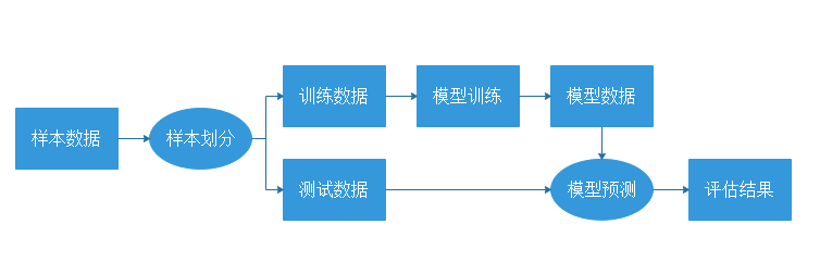
效果验证
效果验证是机器学习非常重要的一个环节,最常使用的是交叉验证。常见的验证过程如图中所示。
以SVM为例,导入SVM库以及Scikit-Learn自带的样本库datasets:
>>> import numpy as np
>>> from sklearn.model_selection import train_test_split
f>>> from sklearn import datasets
>>> from sklearn import svm
获取样本数据:
>>> iris = datasets.load_iris()
>>> iris.data.shape, iris.target.shape
((150, 4), (150,))
为了保证效果,使用函数train_test_spli随机分割样本为训练样本和测试样本:
>>> X_train, X_test, y_train, y_test = train_test_split(
...     iris.data, iris.target, test_size=0.4, random_state=0)
>>> X_train.shape,y_train.shape
((90, 4), (90,))
>>> X_test.shape,y_test.shape
((60, 4), (60,))
调用SVM进行训练:
>>> clf=svm.SVC(kernel='linear',C=1).fit(X_train,y_train)
判断预测结果与测试样本标记的结果,得到准确率:
>>> clf=svm.SVC(kernel='linear',C=1).fit(X_train,y_train)
>>> clf
SVC(C=1, cache_size=200, class_weight=None, coef0=0.0,
  decision_function_shape='ovr', degree=3, gamma='auto', kernel='linear',
  max_iter=-1, probability=False, random_state=None, shrinking=True,
  tol=0.001, verbose=False)
判断预测结果与测试样本标记的结果,得到准确率:
>>> clf.score(X_test, y_test)
0.96666666666666667
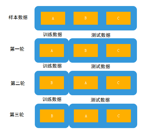
为了提高验证的准确度,比较常见的方法是使用K折交叉验证。所谓K折交叉验证,就是初始采样分割成K个子样本,一个单独的子样本被保留作为验证模型的数据,其他K-1个样本用来训练。交叉验证重复K次,每个子样本验证一次,平均K次的结果或者使用其他结合方式,最终得到一个单一估测。三折交叉验证原理图见下图。
这个方法的优势在于,同时重复运用随机产生的子样本进行训练和验证,每次的结果验证一次,十字交叉验证是最常用的。还是上面的例子,十折交叉法实现如下:
>>> from sklearn.model_selection import cross_val_score
>>> clf = svm.SVC(kernel='linear',C=1)
>>> scores = cross_val_score(clf, iris.data, iris.target, cv=5)
>>> scores
array([ 0.96666667,  1.        ,  0.96666667,  0.96666667,  1.        ])